Proximal Policy Optimization 是一個 fine-tune Model 的方式, 另一個主流方式是 DPO (Direct Preference Optimization). 這邊主要是整理課程影片中 PPO 的公式 (只用大約 2 分鐘超高速閃過…), 以便有空時可以查詢.
[基本架構]
有一個 LLM model, 和可調整的參數: θ, query: X, response: Y, 所有輸出入組合 rollout 表示為 (X, Y).
因為我們要微調這個 model, 所以要給一個獎勵函數 (reward function): r(X,Y), 用來調整模型 πθ (X,Y).
獎勵是對所有輸出的 Y 取期望值
EY~πθ (X,Y) [r(X,Y)], 其中 Y~πθ (X,Y), 表示 Y 在 πθ (X,Y) 的輸出組合.
也對每個 query X 計算
EX~D [EY~πθ (X,Y) [r(X,Y)]] ——————— (1)
其中 X~D , D 表示 X 的散度 (Divergence), 依此類推.
我們找出一個得到最多獎勵的那組參數, 就算是 fine-tune 完成.
π* (X,Y) = arg maxπ {EX~D [EY~πθ (X,Y) [r(X,Y)]]}, {} 裡面就是上面那包.
[Reference model]
做得好不好, 我們要有一個 reference model 來當評審.
πref (X,Y)
Model 的輸出愈接近 reference model 就表示學得愈好.
[懲罰值]
KL 是 Kullback-Leibler 兩個人名的縮寫. KL penality coefficient 是它們衡量懲罰的函數. 基於 reference model πref (X,Y) 下, 對 πθ (X,Y) 產生的懲罰 DKL 表示為
DKL [πθ (X,Y) || πref (X,Y)]
[綜合期望值和懲罰值]
π* (X,Y) = arg maxπ {EX~D [EY~πθ (X,Y) [r(X,Y)]] – β * 懲罰值} =>
π* (X,Y) = arg maxπ {EX~D [EY~πθ (X,Y) [r(X,Y)]] – β DKL [πθ (X,Y) || πref (X,Y)]}
為了要知道往哪個方向調整, 我們要找 θ 的梯度.
[只看 reward function]
這是 reward function 在特定 model 參數 θ 的期望值
E[rY |θ ] = EY~πθ (X,Y) [r(X,Y)]
將它表示為解析函數 [1], 期望值等於所有 Y 可能的值乘上它的機率的和
E[rY |θ ] = ∑Y r(X,Y)πθ (Y|X) —— (2)
最優化的參數 θ⌃ 就是所有 θ 中 reward 最好的. (我打不出 hat theta, 所以把帽子放右邊)
θ⌃ = arg maxθ [E[rY |θ ]] = arg maxθ [∑Y r(X,Y)πθ (Y|X)]
對式子 (2) 取 θ 的梯度,
∇θ E[rY |θ ] = ∑Y r(X,Y) ∇θ πθ (Y|X)] ——– (3)
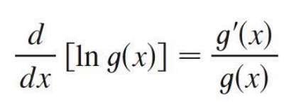
按照微積分的 chain rule [3]
∇θ log (πθ (Y|X)) = ∇θ πθ (Y|X) / πθ (Y|X) =>
∇θ πθ (Y|X) = ∇θ log (πθ (Y|X)) * πθ (Y|X) —– (4)
把這個變長的 (4) 帶回去 (3),
∇θ E[rY |θ ] = ∑Y r(X,Y) ∇θ πθ (Y|X)] =>
∇θ E[rY |θ ] = ∑Y r(X,Y) ∇θ log (πθ (Y|X)) * πθ (Y|X) =>
∇θ E[rY |θ ] = EY~πθ (Y|X) r(X,Y) ∇θ log (πθ (Y|X))
再把 X 考慮進去, 就得到
Ex~D [∇θ E[rY |θ ] ] = ∇θ Ex~D [ E[rY |θ ] ]
意思是說, 當 β = 0, 忽略掉懲罰的話, 對式子 (1) 取梯度, 等效只對 reward function 取梯度. 反之亦然.
這有什麼意義呢? 我請 AI 幫我解釋. 我試了幾次都沒有它講得好.
∇θ E[rY |θ ] = EY~πθ (Y|X) r(X,Y) ∇θ log (πθ (Y|X)) 這個結果是 策略梯度定理(Policy Gradient Theorem) [2] 的核心公式。其意義在於:
將梯度轉換為期望形式 :原始梯度需遍歷所有可能的輸出 ∇θ Y (計算量巨大),但此公式表明:梯度可通過從策略 πθ 中採樣 Y 來近似計算。避開解析計算 :無需知道所有 Y 的機率分佈,只需對採樣的 Y 計算 r(X,Y) ∇θ log (πθ (Y|X)) 的平均值。
它與 Monte Carlo Method 的相似處在於: 透過採樣直接估計期望值,無需精確計算所有可能的 Y.
蒙特卡羅方法收斂速度為 O (1/√N ), N 夠大就好. 而窮舉法不可行.
最後再筆記一下懲罰項.
Kullback-Leibler 方法其實是要避免訓練後新的參數和舊的參數偏差太遠. 以至於學會新的東西就忘了舊的 – 災難性遺忘 (Catastrophic Forgetting), 和 reward 無關. 因此討論原理時可以忽略它.
但它對於穩定系統非常重要, 其主要角色是作為正則化項 (Regularizer), 將策略更新限制在信賴域 (Trust Region) 內. 在PPO算法中,KL 散度還會動態調整更新步長. 當 DKL 超過閾值時自動縮小學習率,此設計本質上將 “避免遺忘" 和 “促進學習" 綁定為同一過程。
[REF]
解析函數 – 維基百科,自由的百科全書 https://en.wikipedia.org/wiki/Policy_gradient_method Slide 1