分類: 技術

LCEL 全名 LangChain Expression Language， 是一種描述 LangChain 架構的語言。最大的特徵就是看到 A = B | C | D 這種表示法 – 說明了 LCEL 串接多個可執行單元的特性，是 LangChain 的進階實現。而 ‘|’ 的理解和 Linux 的 pipe 很像，它是非同步的串接。

舉例來說，一個 LLM 的 LangChain 可以表示為：

chain = prompt | LLM model | Output Parser

依序做好這三件事：有方向性的提示、強大的大語言模型、友善的輸出格式，就可以提升使用者體驗。

但是顯然這樣還不太夠，比方說，LLM 需要查一筆它沒被訓練過的資料，在上面的 pipe 就無法做到。換個例子，我想幫 AI 助理取個名字，它也會說好。但是一轉眼什麼山盟海誓都忘光了!

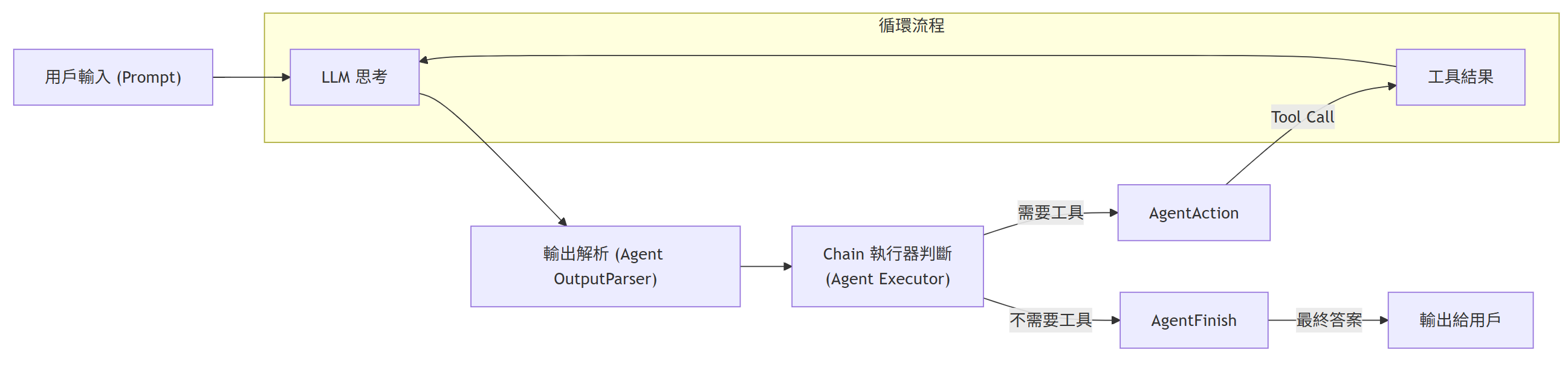
顯然，我們要有個負責的 agent，把 function call 的能力加進來；而且 call 完之後，還要餵給 LLM 做 “人性化" 的自然語言潤飾。這是一個循環的路徑，直到 AI 判斷它不再需要任何外部工具，就可以結束迴圈，跟使用者報告最終結果了。

那麼這個 code 長什麼樣子? 首先把基本元件準備好：

# 初始化模型
llm = ChatOpenAI(model="gpt-4o", temperature=0)

# 將工具打包成列表
tools = [get_current_weather] # 以問天氣的函式為例

# 給出配合 function 的 prompt
prompt = ChatPromptTemplate.from_messages(
    [
        ("system", "你是天氣助理，請根據工具的結果來回答問題。"),
        ("placeholder", "{chat_history}"),  # 預留給歷史訊息
        ("human", "{input}"), # 真正的輸入
        ("placeholder", "{agent_scratchpad}"), # 於思考和記錄中間步驟
    ]
)

創建 agent

# 創建 Tool Calling Agent
# 將 LLM、Prompt 和 Tools 組合起來，處理 Function Calling 的所有複雜流程
agent = create_tool_calling_agent(llm, tools, prompt)

執行 agent

# 創建執行器, 跑 模型思考 -> 呼叫工具 -> 再次思考 -> 輸出答案的循環
agent_executor = AgentExecutor(agent=agent, tools=tools, verbose=True)

設計人機介面

def run_langchain_example(user_prompt: str):
    print(f"👤 用戶提問: {user_prompt}")
    
    # 使用 invoke 運行 Agent，LangChain 會自動管理多輪 API 呼叫
    result = agent_executor.invoke({"input": user_prompt})
    
    print(f"🌟 最終答案: {result['output']}")

測試案例

# 示範一：Agent 判斷需要呼叫工具
run_langchain_example("請問新竹現在的天氣怎麼樣？請告訴我攝氏溫度。")

# 示範二：Agent 判斷不需要呼叫工具，直接回答
run_langchain_example("什麼是 LLM？請用中文簡短回答。")

這邊要留意的是，第一個問天氣的問題，LLM 顯然要用到 tool 去外面問，第二個問題不需要即時的資料，所以它自己回答就好。

意猶未盡的讀者可能好奇 function 長怎樣? 其實就很一般，主要的特色是用 @tool decorator。這樣可以獲得很多好處，最重要的一點是 agent 都認得它的 JSON 輸出，方便資料異步流動。

# LangChain 會自動將這個 Python 函數轉換成模型可理解的 JSON Schema
from langchain_core.tools import tool

@tool
def get_current_weather(location: str, unit: str = "celsius") -> str:
    if "新竹" in location or "hsinchu" in location.lower():
        return "風大啦! 新竹就是風大啦!"
    else:
        return f"我不知道 {location} 的天氣啦!"

另外，追根究柢的讀者可能想問，code 裡面怎麼沒看到 ‘|’? 它跑那裡去了? 沒錯，上面講的都是 agent，它比較進階，可以動態跑流程。反而 LCEL 只是 LangChain 的實行方式，它就是一個線性的 chain。

我們由奢返儉，回過頭來看 LCEL，它不能跟 agent 比，只能打敗傳統的 LangChain。標為紅色的是 LCEL 特色的 coding style。

def demonstrate_legacy_chain():
 
    # 定義模型
    llm = ChatOpenAI(temperature=0)
    
    # 定義 Prompt Template
    template = "Translate English text to Chinese: {text}"
    prompt = PromptTemplate(template=template, input_variables=["text"])
    
    # 建立 Chain (透過類別組合)
    # 缺點：語法較冗長，看不到資料流向，且 output 通常包含原始 meta data
    chain = LLMChain(llm=llm, prompt=prompt)
    
    # 執行
    input_text = "Make American Great Again!"
    result = chain.run(input_text)

VS

def demonstrate_lcel():
    
    # 定義模型
    model = ChatOpenAI(temperature=0)
    
    # 定義 Prompt Template, 使用更現代的 ChatPromptTemplate
    prompt = ChatPromptTemplate.from_template("Translate English text to Chinese: {text}")
    
    # 定義 Output Parser (將 AI Message 轉為純字串)
    output_parser = StrOutputParser()
    
    # 建立 Chain (使用 Pipe '|' 運算符)
    # 優點：Unix 風格管道，由左至右邏輯清晰，易於修改和擴展
    chain = prompt | model | output_parser
    
    # 執行
    input_text = "Make American Great Again!"
    result = chain.invoke({"text": input_text})

這兩個都是一次性的 Q&A。

1. Functions, Tools and Agents with LangChain