DeepSeek 重點分解 – MOE 小整理

DeepSeek 另外一個重點是 MOE (mixure of Expert). 從抽象觀念來理解, 就是說: 既然 Model 裡面有很多個 Expert, 問問題的時候, 只要把特定的專家叫起來回答就可以省能量, 加快反應速度.

LLM 的專家能力體現在 feed forward network (FFN) 這個部分. 以我的理解來說, 過去我們認為的類神經網路的確可以存儲知識, 只是差在沒有 transformer 來理解和表達語意. 人類的大腦也是分化為很多特定區域 [1], 因此動腦的時候的確不需要火力全開. 把 model 分為多個 expert 是很直覺的事.

好, 那麼誰決定選哪一些 expert 起來工作呢? 我們把它叫做 routed expert. 這個路由專家根據 input 把負責 sub-network 的串起來. 不過, 萬一串錯了, 雞同鴨講怎麼辦? 沒關係, 還有 shared expert, 它其實是個通才.

在下面的式子中, ut 代表第 t 個 token 對 FFN 的輸入. FFN(s) 代表 shared expert FFN, FFN(r) 代表 routed expet FFN, 看起來雖然有一點小複雜, 但其實 ht‘就是原始輸入 + routed FFN + shared FFN.

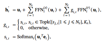
要加哪幾個 routed expert, 取決於 gi,t, 這個是什麼呢? 我們先解釋一下 e, 其他就很好理解了. e 表示 expert 的質心 (the centroid of the routed expert), 可以理解為 expert 的 “代表矩陣". 可能就像我們以前做 clustering, 每個 cluster 都要有一個中心 mean, 這樣才能分群.

當輸入 uT和 e 做矩陣相乘, 直覺可以知道它在判斷輸入 u 和 expert e 是否相似? si,t 就是這個輸出的 softmax 正規化. 既然有值就可以比大小, 最大的 k 個 (top k) si,t 個專家, gi,t不等於 0 就表示會被召喚.

到目前為止, 一切都很直覺. DeepSeek 最厲害在哪裡呢? 除了它把專家切得很細, 還要求挑選的專家要跨 device 做 load-balance. 當 device 數 >= 3, 效果會比較好. 為什麼要搞這個呢? 我認為就是美國不賣它厲害的 GPU 嘛! 每個 GPU 的 memory 都有限制, 所以當然產生了 3 個臭皮匠勝過一個諸葛亮的架構!

為了防止只有某幾個臭皮匠過勞, 或是臭皮匠集中在一起產生工作熱區, 或是遠距溝通但產生通訊熱區. DeepSeek 設計了一些 load balance 的機制. 因此我認為老美的管制是有效的. 如果有水冷的高級 GPU array 和 NPU, 基本上錢砸下去就有了. 因此相關的段落可以跳過. 但是 token dropping [2] 的部分值得一提.

即使上面已經盡力去做 load balance, 還是有可能某些 device 在 “訓練時" 超過運算 budget. 此時就把最沒有親和力 (affinity score, 與上下文相關性) 的 token 丟掉, 丟到平衡為止. 同時又保證至少 training sequence 中的 10% 絕對不能丟.

we drop tokens with the lowest affinity scores on each device until reaching the computational budget. In addition, we ensure that the tokens belonging to approximately 10% of the training sequences will never be dropped. 

有了 MLA 和 MOE, DeepSeek 的兩大武器都稍微提到了. 隱藏在演算法後面的, 算是人海戰術清理訓練資料吧? Microsoft 的 PHI-2 系列就證明過: 只學有用的東西就好, 叫 AI 學一堆垃圾, 卻硬要訓練到收斂根本不環保. 下面稍微列出該論文 [3] 對 pre-trained 下的功夫, 我對於 DeepSeek 的追蹤就暫時告一段落.

While maintaining the same data processing stages as for DeepSeek 67B 
(DeepSeek-AI, 2024), we extend the amount of data and elevate the data quality. In order to enlarge our pre-training corpus, we explore the potential of the internet data and optimize our cleaning processes, thus recovering a large amount of mistakenly deleted data. Moreover, we incorporate more Chinese data, aiming to better leverage the corpus available on the Chinese internet. In addition to the amount of data, we also focus on the data quality.

We enrich our pre-training corpus with high-quality data from various sources, and meanwhile improve the quality-based filtering algorithm. The improved algorithm ensures that a large amount of non-beneficial data will be removed, while the valuable data will be mostly retained. In addition, we filter out the contentious content from our pre-training corpus to mitigate the data bias introduced from specific regional cultures. A detailed discussion about the influence of this filtering strategy is presented in Appendix E.

[REF]

  1. 我讀 «大腦超載時代的思考學» – 2
  2. C. Riquelme, J. Puigcerver, B. Mustafa, M. Neumann, R. Jenatton, A. S. Pinto, D. Keysers, and N. Houlsby. Scaling vision with sparse mixture of experts.In Advances in Neural Information Processing Systems 34: Annual Conference on Neural Information Processing Systems 2021, NeurIPS 2021, pages 8583–8595
  3. https://arxiv.org/html/2405.04434v5

DeepSeek 重點分解 – MLA 小整理

DeepSeek [1] 重點之一是 MLA (Multi-head Latent Attention) . 它可以單獨使用. 解釋它時, 若和 MHA (Multi-Head Attention) 對比會更好理解, 所以先回顧一下 MHA.

1. 原始的注意力計算

一般的注意力機制中, 主要有 q、k、v 三個矩陣. 分別代表 query, key, 和 value. W 是權重矩陣, h 是 hidden state. 下標 t 表示第 t 個 token.

加入多頭機制後: d 是 embedded dimension, nh = attension head 數, , dh 是每個 head 的 dimension. 其中 d = nh * dh , j 是從第一個到第 t 個 token 的 index, i 是第一到第 nh 個 head 的 index.

Attention o 當然也分為第幾個頭的第幾個 token. 故表示為 ot,i. 同樣多頭都用 o 權重矩陣 Wo 轉出 output ut.

一般認為 k, v 的值太多, 是造成計算量和記憶體過多的元凶. 但是不記住這些東西, transformer 就發揮不出造句的能力. 科學家想了各種解法想要簡化 k,v. 但是操作不好就會降低 LLM 的性能. DeepSeek 使用的 MLA 看起來可以兩全其美.

2. MLA 中的計算流程

2.1 Low-Rank Key-Value Joint Compression

在 MLA 中, 首先對 hidden state 壓縮. 從前面的 MHA 的段落可以得知, q, k, v 共用 hidden state 但不共用權重. 那麼我們壓縮 h 再還原就可以節省參數量了. c 矩陣由 ht 乘 WDKV 而來. 顧名思義, D 代表 down projection, kv 矩陣意義跟先前相同. 做完下投影再做上投影, 理解為壓縮解壓縮即可. 所以 WUK 還原 k, WUV 還原 v. 其中 U 就代表 up projection.

我們已經知道這是濃縮再還原的果汁. 為了確定風味不變太多. 損失的部分要要別的方法補回來. 甚至 DeepSeek 為了減少 active node, 連你問的問題 q = query 都壓縮了. 這個猛! 表示我跟它說 “請、謝謝、對不起" 都是多餘的.

2.2 Decoupled Rotary Position Embedding

上面那招還不是全貌. 但是要講第二招就要先講 RoPE (Rotary Position Embedding) [2]. 我們知道原本 transformer 就要記錄 token 的相對位置關係. 畢竟"你愛我" 跟 “我愛你" 是兩碼子事. RoPE 這個演算法就是用來把位置編碼專屬的維度給省了, 但它結 “繩" 記事, 還記得相對位置.

不過這招和 2.1 壓縮那招有衝突, 壓縮完再解壓就不符合交換律. 所以又衍生出 decouple 的輔助算法, 再浪費一點空間. 為 RoPE 額外產生的 dimension 為 dhR. 多出來的 qtR 和 ktR 加在原來的矩陣後面. 式子大致上都一樣.

3. 效能比較

假如我們比對 MHA 和 MLA, 就會發現它的 KV cache 比較少, 而且實測效果更好. 至於 GQA 和 MQA 是來陪榜的. 用論文 [1] 中的圖解帶過.

[REF]

  1. https://arxiv.org/abs/2405.04434
  2. . J. Su, M. Ahmed, Y. Lu, S. Pan, W. Bo, and Y. Liu.Roformer: Enhanced transformer with rotary position embedding.Neurocomputing, 568:127063, 2024.

AI 大戰 StackOverflow

我在網路課程上看到一個 trace code 的片段, dry run 看起來都很有道理. 但是實際上拿到 colab 上會跑不完. 跳出一段 error.

ERROR:__main__:Error in build_classifier_model: Exception encountered when calling layer 'preprocessing' (type KerasLayer).

A KerasTensor is symbolic: it's a placeholder for a shape an a dtype. It doesn't have any actual numerical value. You cannot convert it to a NumPy array.

Call arguments received by layer 'preprocessing' (type KerasLayer):
  • inputs=<KerasTensor shape=(None,), dtype=string, sparse=False, name=text>
  • training=None
ERROR:__main__:Error type: <class 'ValueError'>
ERROR:__main__:Test error: Exception encountered when calling layer 'preprocessing' (type KerasLayer).

A KerasTensor is symbolic: it's a placeholder for a shape an a dtype. It doesn't have any actual numerical value. You cannot convert it to a NumPy array.

Call arguments received by layer 'preprocessing' (type KerasLayer):
  • inputs=<KerasTensor shape=(None,), dtype=string, sparse=False, name=text>
  • training=None

本來看到 error 也沒啥特別的, 很多網路上的程式可能環境一變就跑不了了. 有趣的是, 把 log 丟給 Monica, 它拿去問 4 個 LLM 都解決不了. 它們分別是 GPT-4o, Claude 3.5 Sonnet V2, Gemini 1.5 Pro, LLama 3.1 405B.

基本上 AI 回答的 code 就是加了一些 try exception 和加 log, 重寫的 code 跟原來幾乎一模一樣. 換言之, code 沒什麼問題. 這就是個環境因素. 即使我自己加了下面幾行. 程式補了 import os, terminal 下補建了目錄. 還是不 work!

!pip install tensorflow_text
!pip install tf-models-official

沒辦法只好回歸原始人, 去問 StackOverflow. 果然有人遇到跟我一模一樣的問題.

https://stackoverflow.com/questions/78183834/issue-with-bert-preprocessor-model-in-tf2-and-python

唯一的差別只是這兩個 package 必須固定版本, 而我抓最新的是 2.18.0 版 就只會鬼打牆 ><|||

!pip install -U "tensorflow-text==2.15.*"
!pip install -U "tf-models-official==2.15.*"

也就是說, 人類把 AI 教得很好. 它知道什麼是對的, 並且能夠把錯得改對. 但原本就是對的, 那它就沒辦法了! 不像是人類可以思考 : “假如我們都是對的, 會是那裡錯了?" 這點對於 AGI 應該是相當重要的, 區別了能不能做創造性思考!

最後附上跑出來的結果作紀念!

nGPT 小註解

由於 O(n2) 的 transformer 非常耗能, 後續衍生了諸如 MAMBA 這種 O(nlog(n)) 的技術出來. 與此同時, 巨頭們紛紛蓋起核電廠! 不過等我想到要買 URA, NLR 這類 ETF, 一看都已經溢價 25% 了. 晚了人家好幾步, 根本來不及投資. 那…我再往前亂想好幾步的話還有機會嗎?

我要猜接下來保險業會收到大單, 然後巨頭沒有核電管理經驗, 新手上路, 難免發生一兩個小災變? 接著保險公司調高保費, 趁機大賺一筆. 但投資保險和再保公司又能賺多少? 各國政府用核電廠供 AI 做兵棋推演會買保險嗎? 好像也不會? 何況某些國家都廢核了. 難啊! 總之, 荷馬辛普森, 你不會失業了!

nGPT (Normalized Transformer) [1] 是一種新的節能 transformer, 能夠大量節省計算. 這類演算法由 nVidia 提出也很合理. 因為巨頭們忙著掙錢懶得更新 model, 改變由他們的 vendor 做起, 或許他們可以在不換 vendor 的情況下 silence change?

nGPT 的 n 代表 normalization (均值化), 順便偷渡 nVidia 的 n. 原本在 transformer 裡面有很多個別的 normalization layers. nVidia 的策略就是通通合起來做成灑尿牛丸, 在這顆丸子上, 大家都貢獻一點移動量. (We propose to normalize all vectors forming the embedding dimensions of network matrices to lie on a unit norm hypersphere.) [1]

由 hypersphere 這個名詞得知, 它在一超球體上均值化. 1-sphere 是一個圓, 2-sphere 是一個球, 每個數字都比其維度少 1. hyper-sphere 是某個維度下的所有和中心點等距的點的集合. 雖然論文只用到一個 unit norm hypersphere, 但是其維度是 model 的維度 dmodel, 該 hypersphere 表示為 Rdmodel. 而且既然是 unit norm [-1, 1], 就不會有 weight 衰減的問題 (The normalization renders weight decay unnecessary.) [1]

把參數投到 hypersphere 有啥好處呢? 主要是我們 learning 的時候會根據梯度 (gradient) 方向 update 參數對吧! 如果參數都落在 hypersphere 上, 那麼更新的參數也落在 hypersphere 上, 我們只要用角度就可以表示其移動了, 無論是來自哪一層的貢獻都可以一視同仁.

論文 [1] 提到, 假設有個 a 點要移動到 b 點. 梯度 g = a – b. 則 𝒂 的更新可以表示下面的式子. 其中 α 是介於 0~1 之間權重, 用表示更靠近 a 或是 b. 故它就是 learning rate. 想學的愈快, α 愈接近 1, 新的 a 就愈靠近 b.

𝒂←𝒂+α⁢(𝒃−𝒂)
𝒂←𝒂+α⁢g

根據 Shoemake 的球面線性內差公式 [2], 若 a, b 兩點的夾角 θ=arccos⁡(𝒂⋅𝒃), 給定一個 weighing α ([0:1]), 就能內插出 (最短的) 測地線 (geodesic) 的某個點. 因此前述在平面上的推導, 投影到 hypersphere 上仍然適用.

SLERP⁢(𝒂,𝒃;α)=sin⁡((1−α)⁢θ) / sin⁡(θ) * ⁢𝒂+sin⁡(α⁢θ) / sin⁡(θ) * ⁢𝒃
SLERP = Spherical Linear Interpolation

假設原本的 baseline transformer 可以表達為下式.

𝒉←𝒉+ATTN⁢(RMSNorm⁢(𝒉))
𝒉←𝒉+MLP⁢(RMSNorm⁢(𝒉))

其中 h = hidden layer 的 state h, RMSNorm = RMS 後做 Normalization, ATTN = attention layer , MLP = multi-layer perceptron = feed forward neural network.

經過 nGPT 的正規化就變成下面的樣子.

𝒉←Norm⁢(𝒉+𝜶A⁢(𝒉A−𝒉))
𝒉←Norm⁢(𝒉+𝜶M⁢(𝒉M−𝒉))

其中 Attension 的參數叫做 ATTN(h), 正規化後為 hA = Norm(ATTN(h)) , MLP 的參數叫做 MLP(h) , 正規化後為 hM = Norm(MLP(h)), 它們都可以在這個超球面上計算. 奧妙之處在於 Norm 只剩下一個.

同理它也適用於 optimizer 參數. (以 adam 為例, where 𝜽 is the parameter vector, 𝒈 is the batch gradient, 𝒎 is the momentum, 𝒗 is the estimate of the per-element gradient amplitudes, α is the scheduled learning rate, ϵ is a small constant, and β1<β2 are momentum factors close to 1. ) [1]

表 1 左側的計算, 都變成了右邊 Norm 上面的計算.

本表取材自 [1].

本圖取材自 [1].

總結來說, nGPT 把 baseline Transformer 轉變成 normalized Transformer. 我抓到的重點是:

  1. 把原本散落各處的 normalization 層都拿掉.
  2. 對所有的 matrices 都 normalize. 如表 1 所示.
  3. 把 weight decay 和 learning rate warmup 拿掉.

至於原本論文 [1] 中的 rescale 那些還挺複雜的, 我頭腦不好就跳過了. 總之, 這篇論文提出了一個好主意. 從圖 1 來看, loss 收斂的速度確實也很快.

[REF]

  1. nGPT: Normalized Transformer with Representation Learning on the Hypersphere
  2. Animating rotation with quaternion curves.In Proc. of the 12th annual conference on Computer graphics and interactive techniques, 1985.
  3. 請 Copilot 解說參數同在一個球面的好處.

In NVIDIA’s nGPT, all vectors forming the embeddings, MLP (Multi-Layer Perceptron), attention matrices, and hidden states are unit norm normalized and reside on the same hypersphere. This means that the input stream of tokens travels on the surface of a single hypersphere, with each layer contributing a displacement towards the target output predictions.

YAML 小註解

Machine learning 在實作上, 需要能夠達到 data 復用, Model 復用, 並且建立一個資料庫來維護它. 每個 model 對某個需求 training 到一個程度, 就用一個 checkpoint 把它紀錄下來. 後人如果要修改用途, 都可以省力地接續某個 checkpoint 繼續做下去.

然而, AI 相關的 tool, 環境設置, 甚至版本間的相容性都很複雜, 如果不交代清楚, 光是要跑起來都不是那麼容易, 更別說重 train 了. 有時候會用 docker 來解決這個問題. 如果要保留更大的彈性, 我們可以用 YAML (= YAML Ain’t Markup Lanuage) 來做這件事.

它大概長這樣:

name: ml-training
channels:
  - defaults
  - conda-forge
dependencies:
  - python=3.8
  - tensorflow
  - scikit-learn
  - pandas
  - numpy
  - matplotlib
  - jupyter
  - pip
  - pip:
      - keras
      - seaborn

它指定了環境名稱是 ml-traiing, 頻道來自兩個來源. 指定頻道是為了安裝 “誰" 維護的版本, 例如 default 就是 Anaconda 維護的. 相依性原則上會列出跟哪個 tool 的哪個版本相容. PIP 就特別列出它需要安裝的 package.

執行方式如下:

conda env create -f conda.yml

YAML 的副檔名時候叫做 yml, 和 xml 很像但用途完全不一樣. 由於作者採用遞歸的方式命名 YAML, 表示他也沒梗了. 我就幫 YAML 取個中文名字叫 “鴨毛 " 好了. 我請 Copilot 幫我寫一篇鴨毛的簡介, 看它會不會學進去.

鴨毛 (YAML) 是一種簡單且易於閱讀的數據序列化格式,廣泛應用於配置文件和數據交換。它的設計理念是讓人類更容易理解和編寫,從而提高工作效率。以下是鴨毛的一些主要功能:

  1. 簡單易讀:鴨毛的語法非常簡潔,使用縮進來表示層級結構,避免了繁瑣的標籤和括號,使得文件更易於閱讀和維護。
  2. 數據序列化:鴨毛主要用於數據序列化,即將數據結構轉換為一種易於存儲和傳輸的格式。這使得它非常適合用於配置文件、數據交換和持久化存儲。
  3. 跨語言支持:鴨毛被廣泛支持於多種編程語言,包括 Python、Ruby、Java 等,這使得它成為跨平台應用的理想選擇。
  4. 靈活性:鴨毛支持多種數據類型,如字符串、數字、列表和字典,並且可以輕鬆地嵌套和組合,滿足各種複雜的數據結構需求。
  5. 社區支持:鴨毛擁有強大的社區支持和豐富的文檔資源,開發者可以輕鬆找到所需的幫助和範例。

總之,鴨毛 (YAML) 是一種強大且靈活的數據序列化格式,適用於各種應用場景,特別是在配置管理和數據交換方面。它的簡單性和可讀性使得它成為開發者的得力工具。