DeepSeek [1] 重點之一是 MLA (Multi-head Latent Attention) . 它可以單獨使用. 解釋它時, 若和 MHA (Multi-Head Attention) 對比會更好理解, 所以先回顧一下 MHA.
1. 原始的注意力計算
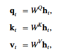
一般的注意力機制中, 主要有 q、k、v 三個矩陣. 分別代表 query, key, 和 value. W 是權重矩陣, h 是 hidden state. 下標 t 表示第 t 個 token.
加入多頭機制後: d 是 embedded dimension, nh = attension head 數, , dh 是每個 head 的 dimension. 其中 d = nh * dh , j 是從第一個到第 t 個 token 的 index, i 是第一到第 nh 個 head 的 index.
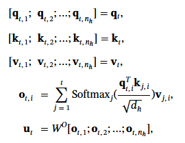
Attention o 當然也分為第幾個頭的第幾個 token. 故表示為 ot,i. 同樣多頭都用 o 權重矩陣 Wo 轉出 output ut.
一般認為 k, v 的值太多, 是造成計算量和記憶體過多的元凶. 但是不記住這些東西, transformer 就發揮不出造句的能力. 科學家想了各種解法想要簡化 k,v. 但是操作不好就會降低 LLM 的性能. DeepSeek 使用的 MLA 看起來可以兩全其美.
2. MLA 中的計算流程
2.1 Low-Rank Key-Value Joint Compression
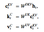
在 MLA 中, 首先對 hidden state 壓縮. 從前面的 MHA 的段落可以得知, q, k, v 共用 hidden state 但不共用權重. 那麼我們壓縮 h 再還原就可以節省參數量了. c 矩陣由 ht 乘 WDKV 而來. 顧名思義, D 代表 down projection, kv 矩陣意義跟先前相同. 做完下投影再做上投影, 理解為壓縮解壓縮即可. 所以 WUK 還原 k, WUV 還原 v. 其中 U 就代表 up projection.
我們已經知道這是濃縮再還原的果汁. 為了確定風味不變太多. 損失的部分要要別的方法補回來. 甚至 DeepSeek 為了減少 active node, 連你問的問題 q = query 都壓縮了. 這個猛! 表示我跟它說 “請、謝謝、對不起" 都是多餘的.

2.2 Decoupled Rotary Position Embedding
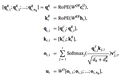
上面那招還不是全貌. 但是要講第二招就要先講 RoPE (Rotary Position Embedding) [2]. 我們知道原本 transformer 就要記錄 token 的相對位置關係. 畢竟"你愛我" 跟 “我愛你" 是兩碼子事. RoPE 這個演算法就是用來把位置編碼專屬的維度給省了, 但它結 “繩" 記事, 還記得相對位置.
不過這招和 2.1 壓縮那招有衝突, 壓縮完再解壓就不符合交換律. 所以又衍生出 decouple 的輔助算法, 再浪費一點空間. 為 RoPE 額外產生的 dimension 為 dhR. 多出來的 qtR 和 ktR 加在原來的矩陣後面. 式子大致上都一樣.
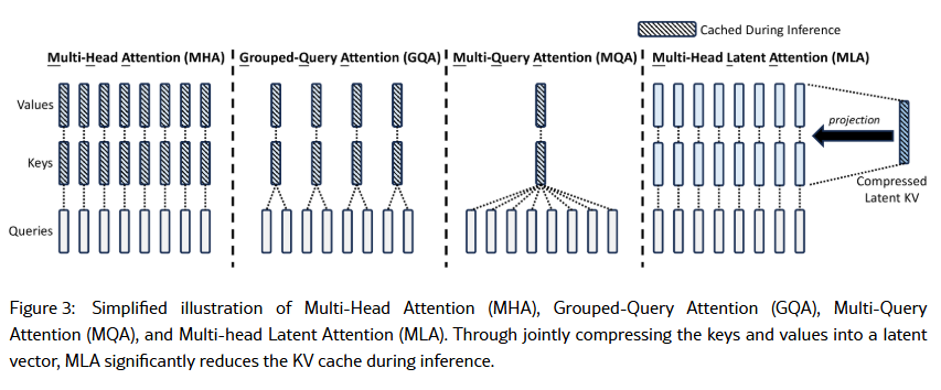
3. 效能比較
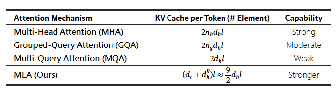
假如我們比對 MHA 和 MLA, 就會發現它的 KV cache 比較少, 而且實測效果更好. 至於 GQA 和 MQA 是來陪榜的. 用論文 [1] 中的圖解帶過.
[REF]
- https://arxiv.org/abs/2405.04434
- . J. Su, M. Ahmed, Y. Lu, S. Pan, W. Bo, and Y. Liu.Roformer: Enhanced transformer with rotary position embedding.Neurocomputing, 568:127063, 2024.