先前分析了 V2 的主力武器, 但 V3 還是比 V2 厲害一截. 所以來談一下 V3 新增的 multi-token prediction (MTP). 雖然 V3 還有厲害的 pre-train 和 fine tune, 但那部份無法用數學或是圖形表示, 只好略過.

本圖取材自 https://github.com/deepseek-ai/DeepSeek-V3
顧名思義, multi-token prediction 就是一次預測好幾個 token. 問題來了, 究竟是一次預測好幾個 tokens (下圖左)?還是預測完一個繼續預測下一個 (下圖中)?還是一次預測好幾個又連續預測好幾步 (下圖右)?

本圖取材自 https://arxiv.org/html/2410.03132v3
其實眼尖一點就可以看到上圖右 (Ours) 一定是該論文認為最好的. 但是這種暴力美學好像跟 DeepSeek 省吃儉用的調性不合. 我們來看看下圖的 DeepSeek V3 架構又是怎做的?
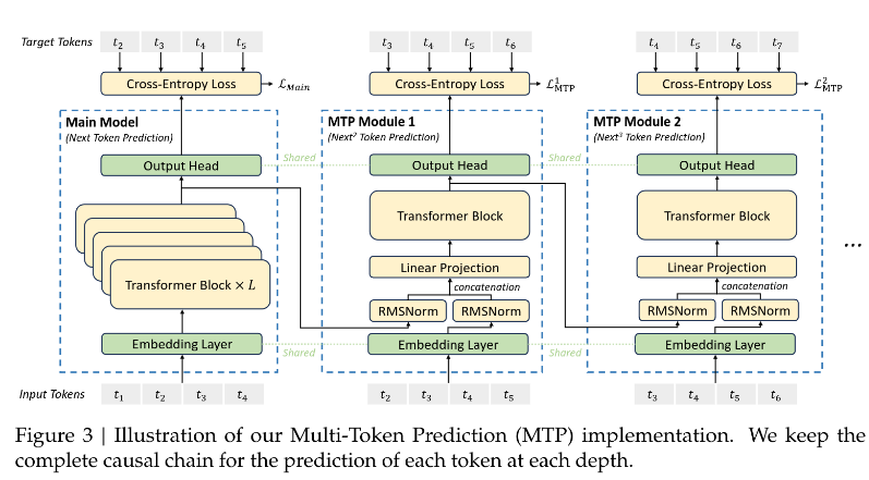
本圖取材自 https://github.com/deepseek-ai/DeepSeek-V3/blob/main/DeepSeek_V3.pdf
我們輸入的 token 是上圖下方的 input t1, t2, t3,… 這些 token, 預測的輸出是上圖上方的 t2, t3, t4….等. 如果我們放置愈多的 MTP module, 就可以預測更深的深度 (Depth). 例如 D = 2, 就是用 t1 預測 t2 和 t3, 用 t2 預測 t3 和 t4, 依此類推. D 愈大, 預測的深度就愈長, 因此它符合 MTP in a single step.
可是一次要預測好幾個 token, 計算不會很大嗎?PDF 提到, 圖裡面的 embedding layer, Output head 雖然畫了好幾個, 但他們都是公用的 (shared).
當我們預測 t2時, 看向上面圖中的 MTP module 1 . 它有且只有兩個輸入, 一個是 t2 經過 embedding, 一個是 t1 在 main Model 的產出物.
至於預測 t3時, 看向上面圖中的 MTP module 2. 它有且只有兩個輸入, 一個是 t3 經過 embedding, 一個是 t2 在 MTP Module 1 的產出物.
因此 D 愈大, 計算的確愈多, 並且有額外的 latency. 但是額外增加的幅度並不等效於再重複一次 main model. 而且這樣有一個好處, 就是 training 時可以好好吸收長距離依賴 (long-range dependencies), 因為它每個預測都以過去歷史為本, 不會即興創作.
至於 multi-token prediction in multiple steps (Autoregressive Chunking) 的方法, DeepSeek 認為在 inference 時確實比較好. 但是在 training 的時候, MTP in one step (Action Chunking) 比較能控制因果關係和長距離依賴.
好!不愛數學的可以停在這裡. 接下來是講公式的部份. 其實跟上面一模一樣, 只是 step 3 增加了以logits 做 softmax() 去字典找字.
Step 1: Combining Representations
For the 𝑖-th input token 𝑡𝑖 at the 𝑘th prediction depth:
- The representation of the 𝑖th token at the (𝑘−1)th depth, denoted as
h𝑘−1i∈ ℝ^𝑑, is taken. If 𝑘 = 1,h𝑘−1𝑖is the representation provided by the main model. - The embedding of the (𝑖+𝑘)th token,
Emb(𝑡𝑖+𝑘) ∈ ℝ^𝑑, is computed using the shared embedding layer. - Both
h𝑘−1𝑖andEmb(𝑡𝑖+𝑘)are normalized using RMSNorm (Root Mean Square Normalization). - The normalized representations are concatenated (
[·; ·]) and linearly projected using the projection matrix𝑀𝑘:- h′ki= Mk[RMSNorm(hk−1i); RMSNorm(Emb(ti+k))].
- Here,
h′𝑘𝑖is the combined representation that serves as the input to the Transformer block at the 𝑘th depth.
Step 2: Transformer Block
The combined representation h′𝑘𝑖 is passed through the 𝑘th Transformer block (TRM𝑘(·)): h𝑘1:𝑇−𝑘 = TRM𝑘(h′𝑘1:𝑇−𝑘).
This produces the output representation h𝑘𝑖 for the 𝑖th token at the 𝑘th depth. The slicing operation 1:𝑇−𝑘 ensures that the sequence length is adjusted appropriately for each prediction depth.
Step 3: Output Head
The output representation h𝑘𝑖 is passed through the shared output head (OutHead(·)), which:
- Linearly maps
h𝑘𝑖to logits. - Applies the Softmax function to compute the probability distribution over the vocabulary:𝑃𝑘𝑖+𝑘+1 = OutHead(h𝑘𝑖).
- Here,
𝑃𝑘𝑖+𝑘+1 ∈ ℝ^𝑉represents the probability distribution for the (𝑖+𝑘+1)th token, where𝑉is the vocabulary size.
- Here,
最後一個重點來了. DeepSeek 只有在 training 的時候使用 one step MTP. 在 inference 的時候, 用的演算法又有不同. “We can also repurpose these MTP modules for speculative decoding (預言家, 投機演算法) [2] to further improve the generation latency."[1]
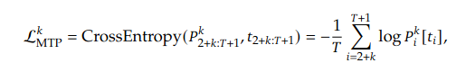
Training 的 loss function 計算也給出來了. 首先, 針對每個 depth (k) 都做計算, P 就是上面的 P. 最後把不同深度的 loss function 取平均值.
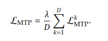
其中 𝜆 當然就是 weighting factor, 或是以前電力機械教授老包所說的 “那麼大”. γ𝜆 = “柑仔那麼大", 是我對這堂課最深的印象.
[REF]
